We get used to the idea that as our sample size increases, our model becomes more reliable.
We all ‘know’ that the sample average of most distributions is asymptotically Normal (by the central limit theorem) and that the sample average gets closer to the population mean and such.
This corresponds to a specific type of randomness, let us call it ‘mild’ randomness, as in a sense nothing wild is going on – although a random (stochastic) process is underneath everything, with more data comes convergence and more reliability to our claims. Our models come from this – linear regression and so on. They are not exact and they accept being approximations, but they still do a decent job.
However, what if they were totally wrong?
Cauchy has a different idea of probability and as a result a different idea of randomness, call it ‘wild’ randomness.
Cauchy’s idea
Cauchy’s idea is as follows.
Consider an archer that is blindfolded and has a bow and arrow. He is to shoot at a target located on a wall that is infinite in height and length. We are to measure how far his arrow is away the target. We assume that he always shoots at the wall, somewhere.
For example. if he hits the target, we record 
We can formulate a probability distribution based on this example and without loss of generality, our assumptions need not hold.
Deriving Cauchy’s distribution
We can represent the idea about the archer above as a right angled triangle, as seen below.
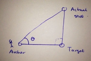
This makes sense when we look at it: we are at some location (labelled archer), say center to the target (labelled target) and some distance (adjacent to the angle 
Then say we are interested in how far we are away from the target (the line segment actual shot – target) and how are we ourselves (the archer) are away from the target (the line segment archer- target). This can be represented by trigonometry and the angle

Let the ratio between the line segment between actual shot and target} and the line segment between archer and target be called 

To measure how far his arrow is away from the target, we are interested in varying

Varying

This derivative defines our distribution – the term 


We then get the probability distribution function defined by integrating
over all real values of 


where
This is the Cauchy distribution.
‘Wild’ randomness
Consider a real life process that conforms to ‘mild’ randomness – the heights of humans, for example.
If I collect heights of say five humans, it may not be close to the average. As I collect more heights I should get closer to the average, assuming that I am picking people randomly and not based on geographical location and other factors.
I get an expected value 

Do these ideas hold for the blinded archer? Well.. not really.
We can have a sequence of shots that are close to the target but if the archer’s next shot is miles away, all that ‘work’ is wiped out in the sense that the average from those previous shots, now considering this shot, will be totally different.
Although I have a ‘bare’ idea on what I expect to get –
Formally this can be shown as the expectation of
The Central Limit Theorem and the Law of Large Numbers do not hold here. Taking the sample average and using it to infer information about this distribution is useless, because the next shot can change all of what we are working with. With the Normal distribution, this is not the case.
Difference between ‘mild’ and ‘wild’ randomness
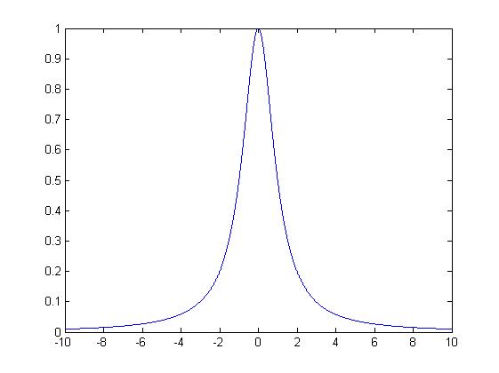
Perhaps the difference between these types of randomness (mild and wild) can be seen in the plots. Consider the plot below of the probability density function of the Cauchy distribution for 

It does not look so much different to the plot of a probability density function of a (standard) Normal distribution, which is plotted below.
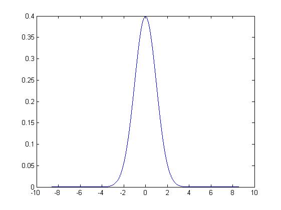
The Cauchy distribution has heavier tails – they do not dip as quickly as they do for the Normal distribution. This corresponds to having a higher chance of an arrow being incredibly away from the target to be more significant in Cauchy’s distribution than in the Normal – this also makes sense. Yet the Cauchy distribution has no (finite) expected value, no (finite) variance and various intuition about it fails – say bye to the Central Limit Theorem and the Law of Large Numbers.


 Posted by AH
  . We know that coin tosses are independent of each other.
 of getting heads (or tails).
 with probability (mass) function
 . The probability mass function is now
 .
. ?
? .
. .
. or any value between zero and one.
 , for
, for  .
. .
.